The story
An office building with 10,000 m² of floor area needs electricity, space heating and cooling. Today it runs on a gas boiler, a chiller and grid electricity. The roof has 2,500 m² for solar panels and the south façade another 200 m².
Which system should it have? Instead of picking one, you give Sympheny the candidates (an air-to-water heat pump, a ground-source heat pump, a gas boiler, a chiller, rooftop and façade solar, a hot-water tank, a cold store and a battery) and let the optimiser decide what to build and at what size.
Because the lowest-cost system is rarely the lowest-emission one, you ask for both: four designs along the trade-off between life-cycle cost and CO₂. Finally you compare them with business as usual. This is the full walkthrough, a remake of our 2021 “Sympheny in 30 minutes” tutorial in the current web app.
Step by step
Follow along in Sympheny. Each step has a screenshot from the video; click the time under it to watch that moment.
- 1
Create the project and its first scenario
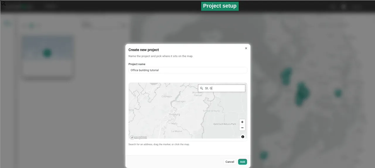
On the projects page, click the plus card. Give the project a name (here Office building tutorial) and click the map to set its location.
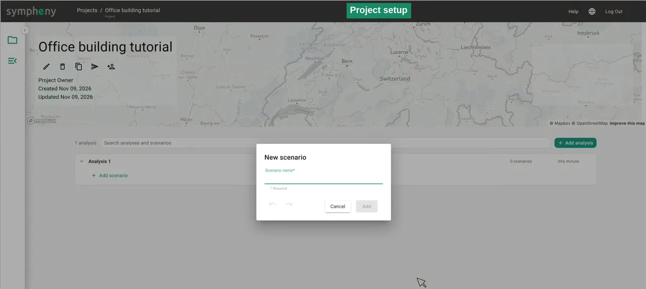
Sympheny creates a first analysis, Analysis 1, and asks for a scenario name. Call it Base case.
Analyses and scenarios structure your study: each scenario is one variant of your system, so you can compare options side by side later.
In the documentation: Projects ↗
- 2
Open the scenario setup
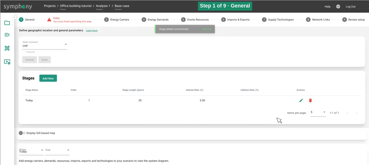
Open the scenario to reach the setup. The nine steps along the top lead from General to Review setup: General, Hubs, Energy Carriers, Energy Demands, Onsite Resources, Imports & Exports, Supply Technologies, Network Links and Review setup.
In the documentation: How the app is structured ↗
- 3
Step 1, General: currency and stage
Keep Swiss francs (CHF) as the currency and add a stage. A stage is a period of time.
Call it Today, give it a duration of 20 years and an interest rate of 3 %. The interest rate discounts future costs, so investments and running costs can be compared over the whole life cycle.
In the documentation: General step ↗ Stages ↗
- 4
Step 2, Hubs: one hub for the building
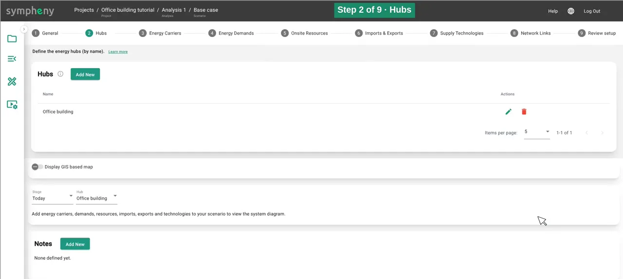
A hub is a node where energy conversion and storage technologies can be installed. It can be a single building, a group of buildings or a whole district.
This study has one hub: Office building.
In the documentation: Hubs step ↗
- 5
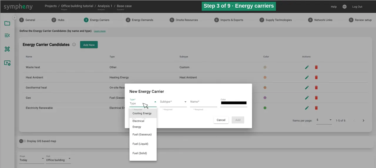
Step 3, Energy Carriers: everything that flows
An energy carrier is any form of energy that flows through the system. Click Add New, pick a Type and a Subtype, and the name is filled in for you. The type only sets the colour; costs and emissions come later.
Add Electricity, Heat 30–40 °C and Cooling 10–20 °C. Then Electricity Renewable, kept separate so you can follow what the solar panels produce, and Gas for a boiler.
Add Geothermal heat and Heat Ambient to feed the heat pumps, a custom carrier called Waste heat for the heat the chiller rejects, and finally solar irradiance for the roof (Solar Roof) and the façade (Solar Facade).
In the documentation: Energy carriers step ↗
- 6
Step 4, Energy Demands: electricity from the database
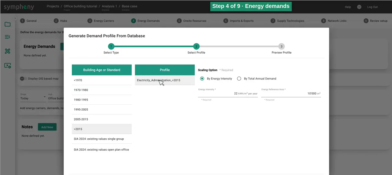
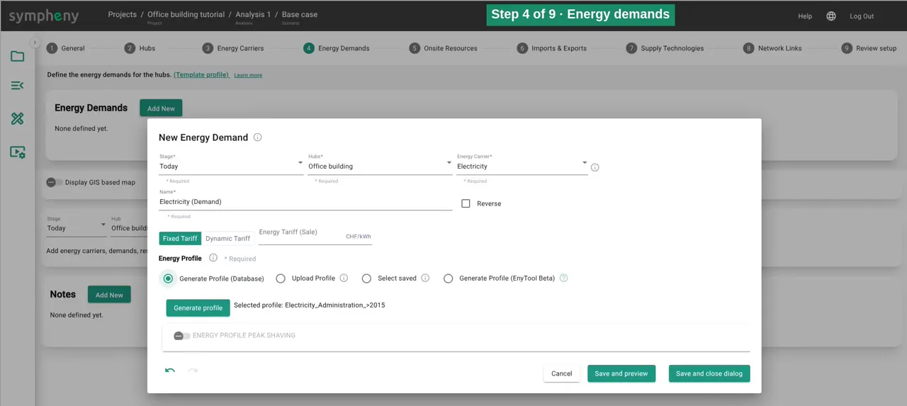
Choose the carrier, Electricity first, and generate an hourly profile from the built-in database: Administration / Office, a building from after 2015 (>2015, profile Electricity_Administration_>2015).
Under Scaling Option choose By Energy Intensity. Clicking the profile fills in the database value, 22 kWh/m² per year; enter 10,000 m² as the Energy Reference Area.
The preview shows 220 MWh a year, with a peak of 110 kW.
In the documentation: Energy demands step ↗
- 7
Step 4, Energy Demands: space heating and cooling
Space heating works the same way: 420 MWh a year, peaking just under 300 kW.
For cooling, use the SIA 2024 standard values for an open-plan office (SIA 2024: existing values open plan office).
You can also upload your own profile with 8,760 hourly values, and the chart icon in the list shows any profile hour by hour.
In the documentation: Energy demands step ↗
- 8
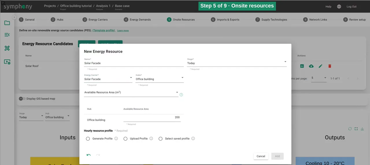
Step 5, Onsite Resources: roof and façade
For the roof, enter the area available for solar panels, 2,500 m², and generate the irradiance profile: St. Gallen, roof, flat.
For the façade, add a second resource: 200 m², vertical (90°), facing south. Each orientation you want to consider gets its own resource.
In the documentation: On-site resources step ↗
- 9
Step 6, Imports & Exports: prices and emissions
Imports and exports set what can enter and leave the site.
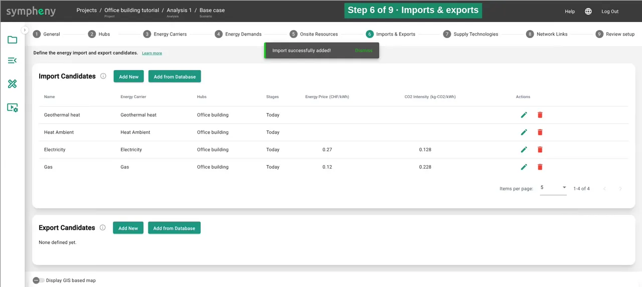
Gas costs 0.12 CHF/kWh and emits 0.228 kg CO₂ per kWh. Grid electricity costs 0.27 CHF/kWh at 0.128 kg CO₂ per kWh.
Ambient heat and geothermal heat are imports too, free of charge: their cost sits in the heat pumps that use them.
On the export side, surplus solar power sells for 0.08 CHF/kWh. Waste heat also needs an exit: every hour has to balance, and the export shows how much heat is released to the surroundings. All prices in this example are illustrative.
In the documentation: Imports & exports step ↗
- 10
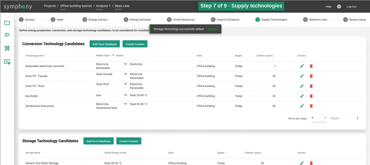
Step 7, Supply Technologies: a custom chiller
Supply technologies are candidates: the optimiser decides whether each one is worth installing, and at what size.
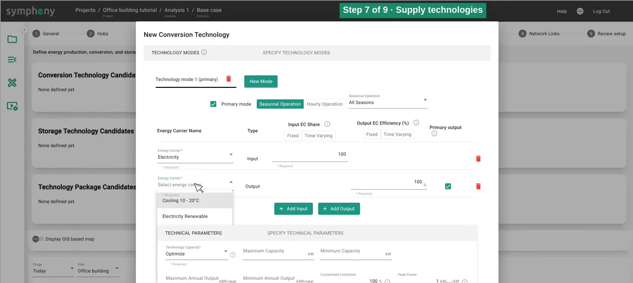
Start with a custom chiller (Create Custom). A technology runs in one or more modes, and each mode turns input carriers into output carriers. The chiller takes electricity and delivers Cooling 10–20 °C at 200 % and Waste heat at 300 %. Efficiencies are relative to the total input.
Leave the capacity to be optimised. Then the costs: a lifetime of 20 years, a fixed investment of about CHF 23,000 plus CHF 938 per kW, and maintenance costs.
In the documentation: Supply technologies step ↗
- 11
Step 7, Supply Technologies: heat pumps and a gas boiler
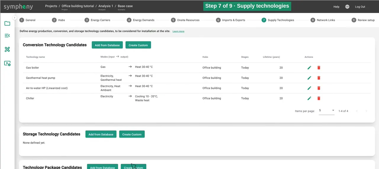
Most technologies can come straight from the database (Add from Database). The air-to-water heat pump comes with costs and performance from the HSLU heating-cost calculator: one part electricity and two parts ambient heat give three parts heat, a COP of 3. Tick it as the Primary mode and add it.
For the ground-source heat pump, take the larger brine-water model, which already includes drilling. Give it a simple name (Geothermal heat pump) and switch its input to your Geothermal heat carrier.
Create the gas boiler yourself: gas in, Heat 30–40 °C out at 95 %, CHF 30,000 plus CHF 110 per kW.
In the documentation: Supply technologies step ↗
- 12
Step 7, Supply Technologies: solar panels and a virtual converter
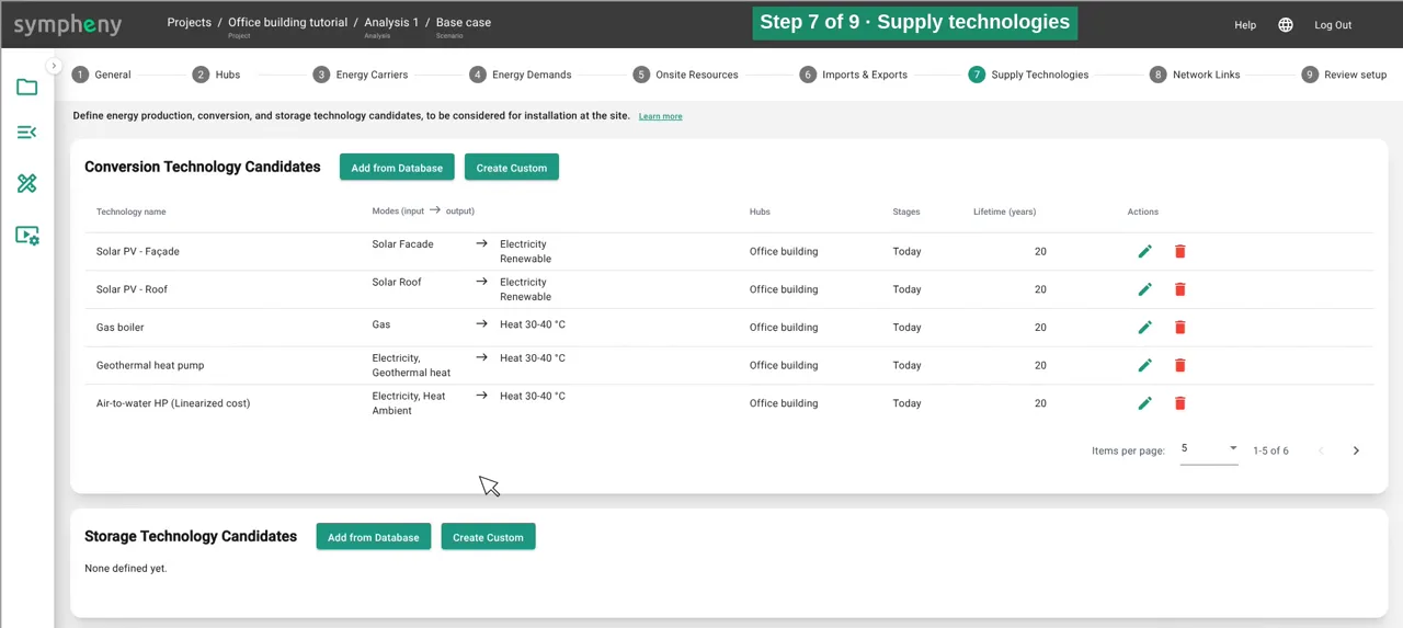
Solar panels for the roof and the façade come from the database (Solar PV - Roof, Solar PV - Façade). Their output becomes Electricity Renewable.
So that this renewable power can also cover the building’s electricity demand, add a virtual technology, Renewable electricity converter. It turns Electricity Renewable into Electricity, with no cost and no losses.
In the documentation: Supply technologies step ↗
- 13
Step 7, Supply Technologies: storage
Add three storages: a hot-water tank, a cold store and a battery.
Database templates sometimes use a carrier you haven’t defined. The hot-water tank expects heat at 70–80 °C, so Sympheny offers to add it. Accept, switch the stored carrier to Heat 30–40 °C, and cap the size at 1,200 kWh so the low-carbon solutions don’t oversize the tank.
The cold store gets 800 kWh. The battery stores Electricity Renewable, up to 1,000 kWh.
In the documentation: Supply technologies step ↗ Storage technologies ↗
- 14
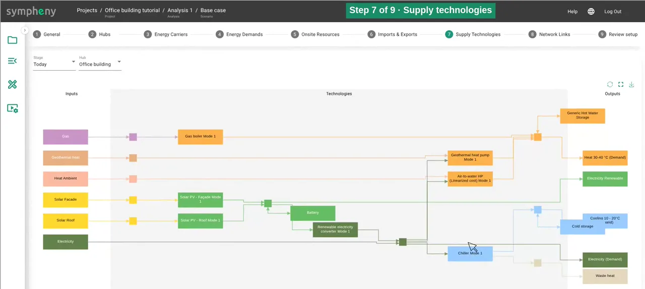
Check the system diagram
Below the lists, the system diagram grows as you go: imports and resources on the left, technologies in the middle, demands and exports on the right. It’s the quickest way to check that everything is connected.
In the documentation: Supply technologies step ↗
- 15
Steps 8 and 9, Network Links and Review setup: run the optimisation
With a single hub, skip Network Links. Review setup lists the whole setup in one place.
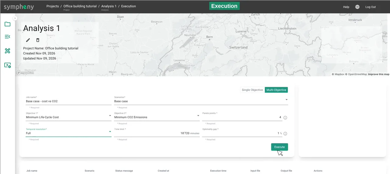
In the execution options choose Multi-Objective, name the job (Base case - cost vs CO2), select the Base case scenario and keep two objectives: Minimum Life-Cycle Cost and Minimum CO2 Emissions.
Set Pareto points to 4: the lowest-cost solution, the lowest-CO₂ solution and two in between. Choose Full temporal resolution (every hour of the year) and click Execute. At full hourly resolution the run takes around ten minutes (this one took about 12).
In the documentation: Network links step ↗ Execution ↗
- 16
Read the results: the Pareto front
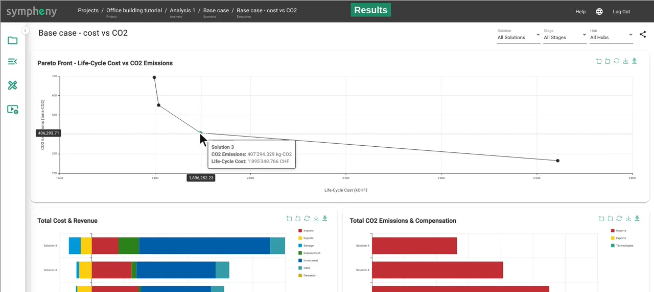
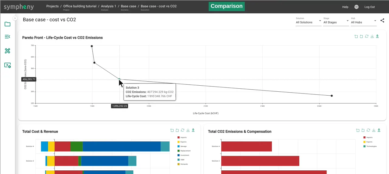
When the run has finished, the results dashboard opens. With all solutions selected, the charts compare the four solutions side by side: investments, installed capacities, storage sizes and annual energy flows.
Set the stage and the hub to All (All Stages, All Hubs) to see the Pareto front: life-cycle cost over 20 years against CO₂ emissions.
Solution 1 is the lowest-cost system: about CHF 1.8 million over 20 years and around 35 tonnes of CO₂ a year. Solution 3 costs only about 5 % more but cuts emissions by about 40 %, to around 20 tonnes a year. Solution 4 gets down to 13 tonnes a year, but costs about CHF 2.6 million.
In the documentation: Results dashboard ↗
- 17
Open solution 3
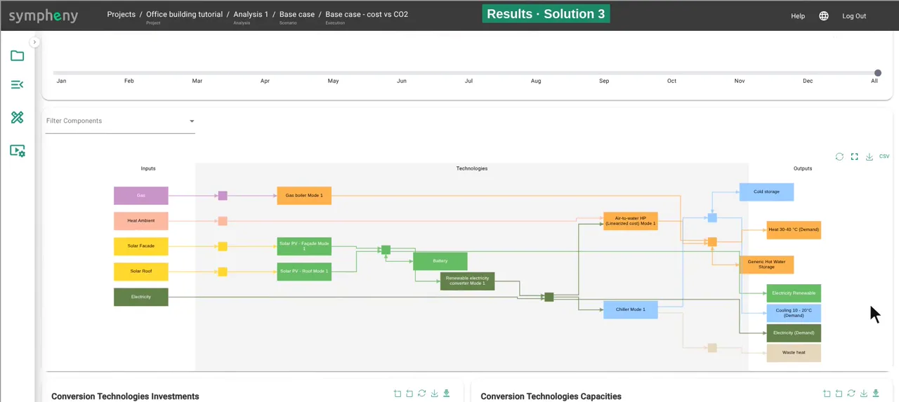
Open solution 3. The Sankey diagram shows every energy flow over the year, and you can filter it by month.
Below, the energy diagram shows what the optimiser chose: an air-to-water heat pump with the gas boiler as back-up, the chiller, solar panels on the whole roof and the façade, and all three storages. The charts underneath give each technology’s investment and capacity.
Why this mix? The heat pump covers almost all of the heat. The gas boiler only helps out on the coldest days, under a hundred hours a year, which costs less than sizing the heat pump for the peak.
From solution 3 to solution 4, each extra tonne of CO₂ avoided gets much more expensive: the last emissions are always the hardest to remove.
In the documentation: Results dashboard ↗
- 18
Build a business-as-usual baseline
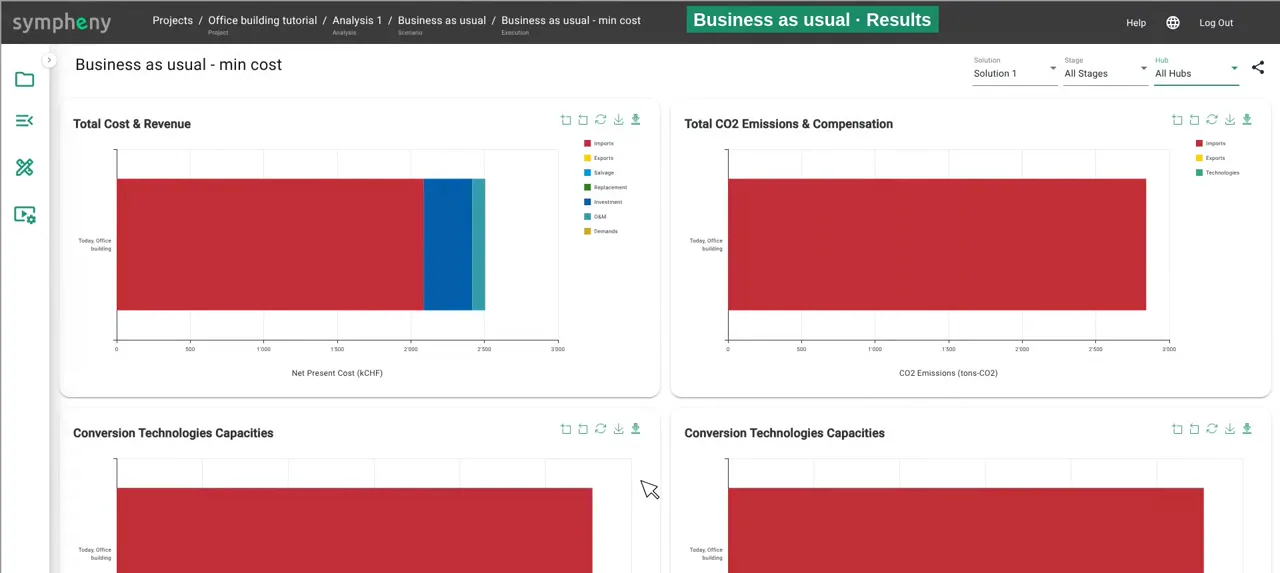
How do these designs compare with the building as it runs today? From the scenario’s ⋮ menu, copy the scenario and call it Business as usual.
Here the gas boiler and the chiller are simply replaced like for like, so delete all the new technology candidates. What’s left is the classic setup: gas for heat and grid electricity for everything else.
Run it for minimum cost (Single Objective). Business as usual costs about CHF 2.5 million over 20 years and emits about 140 tonnes of CO₂ a year.
In the documentation: Analyses and scenarios ↗
- 19
Compare the designs with business as usual
Put the two scenarios side by side. Even the lowest-cost optimised design, solution 1, is about a quarter less expensive than business as usual and cuts emissions by three quarters.
Solution 3 is still about a quarter less expensive than business as usual and cuts CO₂ by more than 85 %.
In the documentation: Results dashboard ↗
Results
Life-cycle cost over 20 years (3 % interest) and CO₂ per year for the four optimised designs and the business-as-usual baseline.
| Life-cycle cost (20 years) | CO₂ per year | vs business as usual | |
|---|---|---|---|
| Business as usual | CHF 2.50 M | 142 t | – |
| Solution 1 (lowest cost) | CHF 1.80 M | 35 t | −28 % cost, −76 % CO₂ |
| Solution 2 | CHF 1.81 M | 28 t | −28 % cost, −81 % CO₂ |
| Solution 3 | CHF 1.90 M | 20 t | −24 % cost, −86 % CO₂ |
| Solution 4 (lowest CO₂) | CHF 2.64 M | 13 t | +5.5 % cost, −91 % CO₂ |
- Every optimised design except the lowest-emission one is about a quarter less expensive than business as usual over 20 years, and all of them cut emissions by at least three quarters.
- Solutions 1 to 3 share the same backbone: an air-to-water heat pump, a gas boiler as back-up, solar on the whole roof and the façade, and three storages. Solution 3 has a bigger heat pump and uses the boiler for under a hundred hours a year.
- The last tonnes are the most expensive: from solution 3 to solution 4 each tonne of CO₂ avoided costs about CHF 5,200, against about CHF 600 from solution 2 to 3. Only solution 4 switches to the ground-source heat pump.
Try it yourself
Build the model alongside the video in your own Sympheny account, then change one assumption and run it again.
Stuck on a step? Ask our support team. Tell us which tutorial and step, and we'll help you get unstuck. Contact support ↗
Video transcript
Here's where we're heading: four optimised designs for one office building, from the lowest-cost system to the lowest-emission one.
Let's build it, step by step.
Welcome to this Sympheny tutorial.
We'll model the building in the Sympheny web app and let the optimiser do the planning.
Everything starts with a project.
I click the plus card, give the project a name, and set its location.
Sympheny creates a first analysis for us and asks for a scenario name.
I'll call it "Base case".
Analyses and scenarios structure your study.
Each scenario is one variant of your system, so you can compare options side by side later.
Opening the scenario takes us to the setup.
The nine steps along the top lead from general settings to the final review.
In General, we keep Swiss francs and add a stage.
A stage is a period of time.
Ours is called "Today", lasts twenty years, and uses a three percent interest rate to discount future costs, so investments and running costs can be compared over the whole life cycle.
Next, hubs.
A hub is a node where energy conversion and storage technologies can be installed.
It can be a single building, a group of buildings, or a whole district.
We have one hub: the office building.
Step three: energy carriers.
An energy carrier is any form of energy that flows through the system.
I pick a type and a subtype, and the name is filled in for me.
The type only sets the colour; costs and emissions come later.
We need electricity, heat at thirty to forty degrees, and cooling at ten to twenty degrees.
Then renewable electricity, kept separate so we can follow what the solar panels produce, and gas for a boiler.
Geothermal heat and ambient heat will feed the heat pumps.
A custom carrier called "waste heat" takes the heat our chiller rejects.
And finally, solar irradiance on the roof and on the façade.
Now the energy demands.
I choose the carrier, electricity first, and generate an hourly profile from the built-in database.
Electricity, administration and office, a building from after 2015.
I scale it by energy intensity.
Clicking the profile fills in the database value, twenty-two kilowatt hours per square metre and year, and I enter ten thousand square metres of floor area.
The preview shows two hundred and twenty megawatt hours a year, with a peak of a hundred and ten kilowatts.
Space heating works the same way: four hundred and twenty megawatt hours, peaking just under three hundred kilowatts.
For cooling, I use the SIA 2024 standard values for an open-plan office.
You can also upload your own profile, with eight thousand seven hundred and sixty hourly values, and the chart icon shows any profile hour by hour.
Step five: onsite resources.
For the roof, I enter the area available for solar panels, two thousand five hundred square metres, and generate the irradiance profile: Saint Gallen, roof, flat.
For the façade, two hundred square metres, vertical, facing south.
Each orientation you want to consider gets its own resource.
Imports and exports set what can enter and leave the site.
Gas costs twelve centimes per kilowatt hour and emits zero point two two eight kilograms of CO2 per kilowatt hour.
Grid electricity costs twenty-seven centimes, at zero point one two eight kilograms.
Ambient heat and geothermal heat are imports too, free of charge.
Their cost sits in the heat pumps that use them.
On the export side, surplus solar power sells for eight centimes.
Waste heat also needs an exit: every hour has to balance, and it shows how much heat we release to the surroundings.
All prices in this example are illustrative.
Step seven: supply technologies.
These are candidates.
The optimiser decides whether each one is worth installing, and at what size.
We start with a custom chiller.
A technology runs in one or more modes, and each mode turns input carriers into output carriers.
Our chiller takes electricity and delivers cooling at two hundred percent and waste heat at three hundred percent.
Efficiencies are relative to the total input.
The capacity is optimised.
Then the costs: twenty years of lifetime, a fixed investment of about twenty-three thousand francs plus nine hundred and thirty-eight francs per kilowatt, and maintenance costs.
Most technologies can come straight from the database.
The air-to-water heat pump comes with costs and performance from the HSLU heating-cost calculator.
One part electricity and two parts ambient heat give three parts of heat, a COP of three.
I tick it as the primary mode and add it.
For the ground-source heat pump, I take the larger brine-water model, which already includes drilling.
I give it a simple name and switch its input to our geothermal heat.
The gas boiler I create myself: gas in, heat out at ninety-five percent, thirty thousand francs plus a hundred and ten francs per kilowatt.
Solar panels for the roof and the façade come from the database.
Their output becomes renewable electricity.
So that this renewable power can also cover the building's electricity demand, I add a virtual technology.
It turns renewable electricity into electricity, with no cost and no losses.
Then storage: a hot-water tank, a cold store and a battery.
Database templates sometimes use a carrier you haven't defined.
The hot-water tank expects heat at seventy to eighty degrees, so Sympheny offers to add it.
I accept, switch the stored carrier to our thirty-to-forty-degree heat, and cap the size at twelve hundred kilowatt hours, so the low-carbon solutions don't oversize the tank.
The cold store gets eight hundred kilowatt hours.
The battery stores renewable electricity, up to a thousand.
Below, the system diagram grows as we go: imports and resources on the left, technologies in the middle, demands and exports on the right.
It's the quickest way to check that everything is connected.
With a single hub, we skip network links.
The review step lists the whole setup in one place.
In the execution options, I name the job, select the Base case, and keep two objectives: minimum life-cycle cost and minimum CO2 emissions.
Four Pareto points give us the lowest-cost solution, the lowest-CO2 solution and two in between.
I run it at full hourly resolution and click Execute.
At full hourly resolution, this run takes about ten minutes.
When the run has finished, the results dashboard opens.
With all solutions selected, the charts compare the four solutions side by side: investments, installed capacities, storage sizes and annual energy flows.
Set the stage and the hub to "All", and you see the Pareto front: life-cycle cost over twenty years against CO2 emissions.
Solution one is the lowest-cost system: about 1.8 million francs over twenty years, and around thirty-five tonnes of CO2 a year.
Solution three costs only about five percent more, but cuts emissions by about forty percent, to about twenty tonnes a year.
Solution four gets down to thirteen tonnes a year, but costs about 2.6 million.
Let's open solution three.
The Sankey diagram shows every energy flow over the year, and you can filter it by month.
Below, the energy diagram shows what the optimiser chose: an air-to-water heat pump with a gas boiler as back-up, the chiller, solar panels on the whole roof and the façade, and all three storages.
The charts underneath give each technology's investment and capacity.
Why this mix?
The heat pump covers almost all of the heat.
The gas boiler only helps out on the coldest days, under a hundred hours a year, which costs less than sizing the heat pump for the peak.
And from solution three to four, each extra tonne of CO2 avoided gets much more expensive.
The last emissions are always the hardest to remove.
But how do these compare with the building as it runs today?
I copy the scenario and call it Business as usual.
Here, the gas boiler and the chiller are simply replaced like for like, so I delete all the new technology candidates.
What's left is the classic setup: gas for heat, and grid electricity for everything else.
I run it for minimum cost.
Business as usual costs about 2.5 million francs over twenty years, and emits about a hundred and forty tonnes of CO2 a year.
So even the lowest-cost optimised design, solution one, is about a quarter less expensive than business as usual, and cuts emissions by three quarters.
Solution three is still about a quarter less expensive, and cuts CO2 by more than eighty-five percent.
That's a complete office building: modelled, optimised, and compared with business as usual.
To try it on your own project, get in touch at sympheny.com.